Tumor
癌症序列变异解释和报告的标准和指南(ASCO和CAP联合推荐)
肺癌分析插件Can_28修复问题
Chom化疗插件及bug修复
Brca插件
FACTERA-fusionGene
SEGF-挖掘NGS中融合基因的新方法
maftools-肿瘤突变数据可视化神器
从数据库中获取免疫相关基因(IRGs)
数据库10KIP—基于ImmPort免疫组学数据挖掘
TCGA数据分析
下载分析TCGA数据库的数据
差异表达分析(limma & edgeR & DESeq2)
TCGA数据的规律【更新中】
生存分析
生存模型构建
突变数据
本文档使用 MrDoc 发布
-
+
up
down
首页
差异表达分析(limma & edgeR & DESeq2)
> TCGA difference analysis generally does not directly use the T test (unless the downloaded FPKM data), but downloads the Counts data and then uses the limma package or the edge package for difference analysis. TCGA 数据分析实战 —— 差异基因 转录组分析中必不可少的差异基因分析,以及通路富集分析 ## 数据准备 下载STAR-Counts和临床信息数据之后,需要分别合并成两个矩阵 ``` # STAR-Counts 数据下载 query_TCGA = GDCquery(project="TCGA-LUSC", data.category="Transcriptome Profiling", experimental.strategy="RNA-Seq", workflow.type="STAR - Counts", access="open") GDCdownload(query = query_TCGA, files.per.chunk = 10) # 临床信息下载 clinical = GDCquery_clinic(project = "TCGA-LUSC", type = "clinical") write.csv(file="clinical.csv", clinical) # 直接使用GDCprepare来获取合并后的数据(保存到文件TCGA_LUSC.rda,便于后续直接使用) lusc.count = GDCprepare(query=query_TCGA, save=TRUE, save.filename="TCGA_LUSC.rda", summarizedExperiment=TRUE) |================================================|100% Completed after 1 m Starting to add information to samples => Add clinical information to samples => Adding TCGA molecular information from marker papers => Information will have prefix 'paper_' lusc subtype information from:doi:10.1038/nature11404 Available assays in SummarizedExperiment : => unstranded => stranded_first => stranded_second => tpm_unstrand => fpkm_unstrand => fpkm_uq_unstrand => Saving file: TCGA_LUSC.rda dim(lusc.count) # 数据整理成表达矩阵用于后续分析 expMatrix = TCGAanalyze_Preprocessing(lusc.count) library(SummarizedExperiment) # SummarizedExperiment(https://bioconductor.org/packages/release/bioc/html/SummarizedExperiment.html) colnames(colData(lusc.count)) # 查看所有列名,81条 table(lusc.count@colData$vital_status) # 查看生命状态情况 table(lusc.count@colData$ajcc_pathologic_stage) #查看肿瘤分期TNM table(lusc.count@colData$definition) #查看肿瘤分类 table(lusc.count@colData$tissue_or_organ_of_origin) #组织来源 table(lusc.count@colData$gender) #性别 table(lusc.count@colData$race) #查看人种 #####gene expression eset dim(assay(lusc.count)) # gene expression matrices. # 60660 553 head(assay(lusc.count)[,1:3]) # expression of first 6 genes and first 3 samples head(rowData(lusc.count)) # ensembl id and gene id of the first 6 genes. # 如前面GDCprepare未保存数据,这儿可以保存该数据到RDS文件中。 saveRDS(object = luad.count, file = "TCGA_LUSC.RDS", compress = FALSE) ``` ## 数据分析 ``` # Load packages library("TCGAbiolinks") library("limma") library("edgeR") library("SummarizedExperiment") library("DESeq2") # load data lusc.count = load(file="TCGA_LUSC.rda") lusc.count = data rm(data) # lusc.count = readRDS(file = "TCGA_LUSC.RDS") # 下面进行临床信息处理 # 提取临床信息 clinical_data = colData(lusc.count) # 获取分组情况 group = factor(clinical_data$definition) levels(group) # 定义 Solid Tissue Normal 类型作为参考。(as being the base or reference level.) group = relevel(group, ref="Solid Tissue Normal") # 创建矩阵 design = model.matrix(~group) head(design) # 生成DGEList对象,用于后续过滤及分析 dge = DGEList( # creating a DGEList object counts=assay(lusc.count), samples=colData(lusc.count), genes=as.data.frame(rowData(lusc.count))) # 过滤 filtering keep = filterByExpr(dge, group=design) dge = dge[keep,,keep.lib.sizes=FALSE] rm(keep) dim(dge) # 可视化 dir.create("./plots") #create folder save_dir <- "./plots/" # 原始reads数绘图 density plot of raw read counts (log10) # dge$samples$lib.size png(paste0(save_dir, "lib_sizes.png"), width=1000, height=900) barplot(dge$samples$lib.size, names=colnames(dge), las=2) # Add a title to the plot title("Barplot of library sizes") dev.off() # 分布分析 # Get log2 counts per million logcounts <- cpm(dge,log=TRUE) # Check distributions of samples using boxplots png(paste0(save_dir, "boxplotslogcpms.png"), width=1000, height=900) boxplot(logcounts, xlab="", ylab="Log2 counts per million",las=2) # Let's add a blue horizontal line that corresponds to the median logCPM abline(h=median(logcounts),col="blue") title("Boxplots of logCPMs (unnormalised)") dev.off() # 标准化calculate normalization factors between libraries dge = calcNormFactors(dge, method="TMM") dge$samples$norm.factors #normalisation by the method of trimmed mean of M-values (TMM) #is performed using the calcNormFactors function in edgeR. #The normalisation factors calculated here are used as a scaling factor for the library sizes. colnames(design) colnames(design)<- gsub(" ", "_", colnames(design)) colnames(design) #verify underscores # normalise the read counts with 'voom' function #incorporate sample-level weights together with the abundance dependent weights estimated by voom v = voom(dge, design, plot=TRUE) v #fit model vfit = lmFit(v, design) efit = eBayes(vfit, trend= TRUE) #sumary tests #Significance is defined using an adjusted p-value cutoff that is set at 5% by default. summary(decideTests(efit)) png(paste0(save_dir, "plotSA.png"), width=1000, height=900) plotSA(efit, main="Final model: Mean-variance trend") dev.off() # 离散评估 y <- estimateDisp(y,design) # quasi-likelihood F-tests fit <- glmQLFit(y,design) qlf <- glmQLFTest(fit,coef=2) ``` ## 使用limma差异分析 ``` library(limma) library(edgeR) ``` ## 1. 数据准备 我们来分析 LGG 和 GBM 之间的转录组差异,首先从 GDC 中获取原位癌 read count 数据 ```R library(TCGAbiolinks) get_count <- function(cancer) { query <- GDCquery( project = cancer, data.category = "Gene expression", data.type = "Gene expression quantification", platform = "Illumina HiSeq", file.type = "results", sample.type = c("Primary Tumor"), legacy = TRUE ) # 选择 20 个样本 query$results[[1]] <- query$results[[1]][1:20,] GDCdownload(query) # 获取 read count exp.count <- GDCprepare( query, summarizedExperiment = TRUE, ) return(exp.count) } gbm.exp <- get_count("TCGA-GBM") lgg.exp <- get_count("TCGA-LGG") dataPrep_GBM <- TCGAanalyze_Preprocessing( object = gbm.exp, cor.cut = 0.6, datatype = "raw_count" ) dataPrep_LGG <- TCGAanalyze_Preprocessing( object = lgg.exp, cor.cut = 0.6, datatype = "raw_count" ) # 合并数据并使用 gcContent 方法进行标准化 dataNorm <- TCGAanalyze_Normalization( tabDF = cbind(dataPrep_LGG, dataPrep_GBM), geneInfo = TCGAbiolinks::geneInfo, method = "gcContent" ) # 分位数过滤 dataFilt <- TCGAanalyze_Filtering( tabDF = dataNorm, method = "quantile", qnt.cut = 0.25 ) # 将数据拆分 dataLGG <- subset(dataFilt, select = gbm.exp$barcode) dataGBM <- subset(dataFilt, select = lgg.exp$barcode) ``` ## TCGA(转录组)差异分析三大R包及其结果对比 [TCGA(转录组)差异分析三大R包及其结果对比](https://mp.weixin.qq.com/s?__biz=MzU4NjU4ODQ2MQ==&mid=2247486990&idx=1&sn=9d1a39962cc9a077eb33048ce0cf718a&scene=21#wechat_redirect) 使用转录组三大R包deseq2,limma和edgeR分别进行差异分析,他们的差异基因可视化如下。 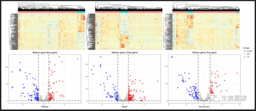 ## 2. edgeR edgeR 可以对 RNA-seq、SAGE 或 ChIP-Seq 等数据进行差异表达分析,任何从基因组特征上产生的 read count 都可以分析 该算法既可以用于多组实验的统计分析,也可以使用广义线性模型(glm)方法来对多因子实验数据进行统计分析 不仅可以应用在基因水平,也可以在外显子、转录本水平进行差异分析,我们以基因水平为例 使用 `TCGAbiolinks` 提供的差异表达分析方法,可以很容易地获取差异基因列表 ```R DEGs.edgeR <- TCGAanalyze_DEA( mat1 = dataLGG, mat2 = dataGBM, Cond1type = "LGG", Cond2type = "GBM", fdr.cut = 0.01 , logFC.cut = 1, method = "glmLRT" ) ```  edgeR 包含许多分析的变体,其中 glm 方法较经典的方法更加灵活,而 glm 方法又包含两种检验方法:似然率检验和准似然率 F 检验,其中准似然率的方法适用于 RNA-seq,似然率检验方法适用于单细胞 RNA-seq 和无生物学或技术重复的数据。 其中 method 参数支持两种方法: glmLRT:似然率检验 exactTest:经典方法,两组间配对均值差的精确检验 也可以使用 edgeR 包提供的函数来识别差异基因 ```R library(edgeR) # 合并 read counts 数据 x <- cbind(dataPrep_LGG, dataPrep_GBM) group <- ifelse(colnames(x) %in% gbm.exp$barcode, 1, 2) y <- DGEList(counts = x, group = group) # 过滤低表达基因 keep <- filterByExpr(y) y <- y[keep,,keep.lib.sizes=FALSE] # RNA-seq 数据,推荐使用 TMM 标准化 y <- calcNormFactors(y) # 构建设计矩阵,由于设置分组 design <- model.matrix(~group) # 离散评估 y <- estimateDisp(y,design) # quasi-likelihood F-tests fit <- glmQLFit(y,design) qlf <- glmQLFTest(fit,coef=2) ``` 准似然率检验的 top 基因 ```R > topTags(qlf) Coefficient: group logFC logCPM F PValue FDR FTHL3 6.199229 3.276914 368.7956 3.511379e-22 5.467568e-18 NACAP1 5.696704 1.979549 282.2026 4.742793e-20 3.692501e-16 LOC728643 5.803125 1.175056 172.4759 2.527741e-16 1.311982e-12 H3F3C 1.966811 4.100946 160.0586 8.745783e-16 3.404515e-12 RPL17 2.141402 6.987182 146.1642 3.856715e-15 1.201058e-11 TMOD2 1.926996 7.926813 135.9716 1.231274e-14 3.195360e-11 RPL13AP3 5.331669 -1.467946 128.9576 2.848142e-14 6.335488e-11 VKORC1 -1.464038 6.009896 125.9088 4.145942e-14 8.069558e-11 LYPLA1 -1.560197 5.911095 124.9255 4.686569e-14 8.108285e-11 CPEB3 2.157688 3.651139 120.9170 7.784031e-14 1.212051e-10 # likelihood ratio tests fit <- glmFit(y,design) lrt <- glmLRT(fit,coef=2) ``` 似然率检验的 top 基因 ```R > topTags(lrt) Coefficient: group logFC logCPM LR PValue FDR FTHL3 6.198600 3.276914 372.0878 6.570886e-83 1.023153e-78 NACAP1 5.696150 1.979549 345.9657 3.203870e-77 2.494373e-73 LOC728643 5.803098 1.175056 273.6598 1.808411e-61 9.386255e-58 RPL13AP3 5.330410 -1.467946 151.4426 8.387839e-35 3.265176e-31 H3F3C 1.966764 4.100946 143.7204 4.090057e-33 1.273726e-29 RPL17 2.141400 6.987182 140.4016 2.174685e-32 5.513899e-29 SLC6A10P 4.275208 -1.038397 140.1416 2.478794e-32 5.513899e-29 TMOD2 1.926998 7.926813 128.9986 6.786503e-30 1.320908e-26 GCSH 3.854903 1.669420 121.2087 3.439727e-28 5.951109e-25 LYPLA1 -1.560212 5.911095 114.7787 8.798646e-27 1.370037e-23 ``` ## 3. limma limma 也是一个可以对芯片和 RNA-seq 数据进行差异表达分析的包,它的线性模型和差异表达函数可以应用于任何基因表达定量技术,也包括定量 PCR,还可以处理单通道和双通道的数据。 limma 包集成了很多功能,包括数据的读取、预处理(如背景矫正、组内或组件标准化等)和差异表达分析 使用 `TCGAanalyze_DEA` 函数,只需指定 pipeline = "limma",便会使用 limma 包中的函数来识别差异表达基因,例如 ```R DEGs.limma <- TCGAanalyze_DEA( mat1 = dataLGG, mat2 = dataGBM, pipeline = "limma", Cond1type = "LGG", Cond2type = "GBM", fdr.cut = 0.01 , logFC.cut = 1 ) ``` 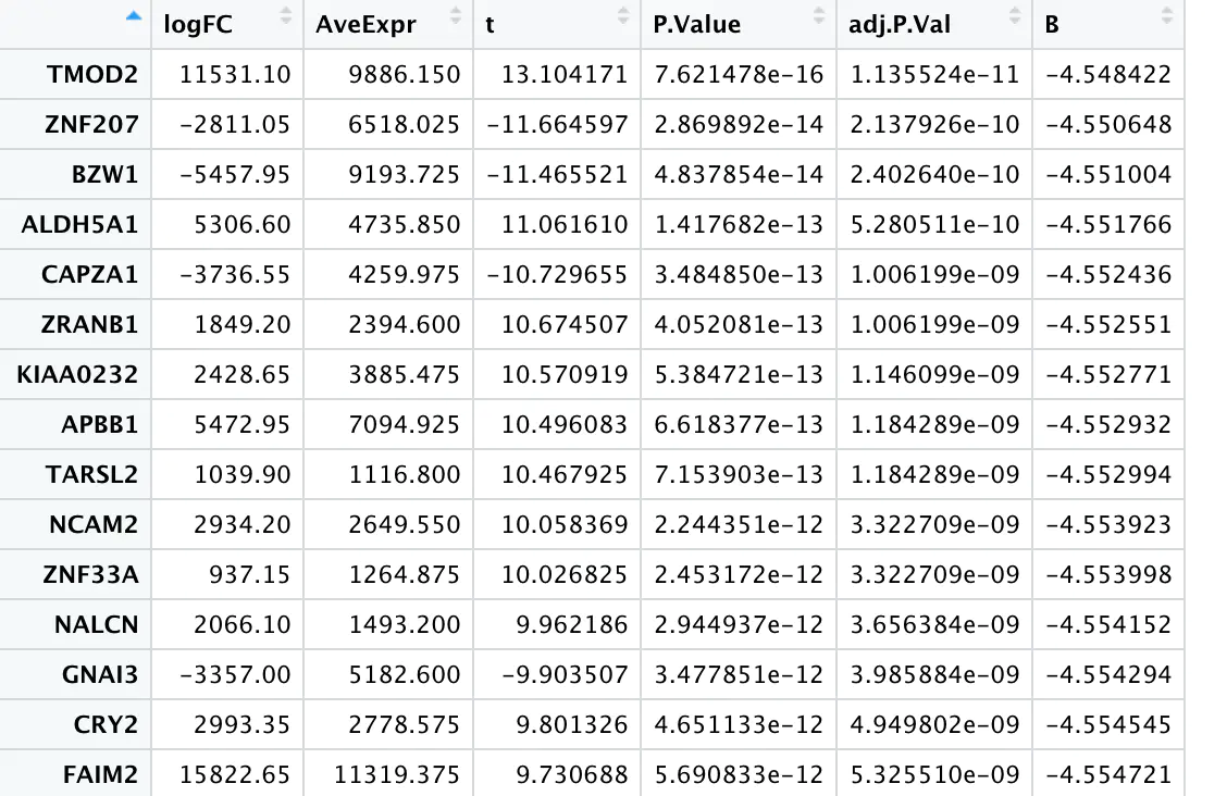 运行上面的代码会返回一张图  如果使用 limma 包来分析,可以先用 edgeR 的几个函数来过滤低表达的基因,然后进行 TMM 标准化,例如 ```R counts <- cbind(dataPrep_LGG, dataPrep_GBM) dge <- DGEList(counts=counts) keep <- filterByExpr(dge, design) dge <- dge[keep,,keep.lib.sizes=FALSE] dge <- calcNormFactors(dge) ``` 如果样本之间的测序深度高度一致,则最简单最鲁棒的方法是使用 limma-trend 来进行差异表达分析。该方法需要使用 edgeR 的 cpm 函数先将 count 数转换为 logCPM `logCPM <- cpm(dge, log=TRUE, prior.count=3)` prior.count 用于控制低 count 的对数方差,获取的 logCPM 值可以应用于任何标准的 limma 流程,例如 ```R fit <- lmFit(logCPM, design) fit <- eBayes(fit, trend=TRUE) topTable(fit, coef=ncol(design)) > topTable(fit, coef=ncol(design)) logFC AveExpr t P.Value adj.P.Val B NACAP1|83955 5.019785 0.2889119 26.09854 1.784215e-27 2.795507e-23 50.54761 FTHL3|2498 5.674651 1.1845469 25.41154 5.094355e-27 3.990918e-23 49.64564 LOC728643|728643 4.654882 -0.4465236 22.68152 4.279208e-25 2.234888e-21 45.76199 GCSH|2653 3.754083 0.4104193 16.75698 3.830152e-20 1.500271e-16 35.31615 SLC6A10P|386757 2.962269 -1.6739395 16.15459 1.446361e-19 4.532316e-16 34.06532 RPL13AP3|645683 2.695707 -2.2357252 14.03958 2.075289e-17 5.419270e-14 29.34302 PPIAL4C|653598 2.681801 -1.3227442 13.72591 4.523101e-17 1.012399e-13 28.59619 TMOD2|29767 2.139542 7.4007515 12.49070 1.090567e-15 2.020331e-12 25.53092 HNRNPA3P1|10151 2.239508 0.7594537 12.46728 1.160517e-15 2.020331e-12 25.47083 RPL17|6139 2.173207 6.5201863 12.32842 1.680040e-15 2.632287e-12 25.11311 ``` 可以在对基因排序时,给 FC 添加更高的权重 ```R fit <- lmFit(logCPM, design) fit <- treat(fit, lfc=log2(1.2), trend=TRUE) ``` ```R > topTreat(fit, coef=ncol(design)) logFC AveExpr t P.Value adj.P.Val NACAP1|83955 5.019785 0.2889119 24.73099 7.502004e-27 1.175414e-22 FTHL3|2498 5.674651 1.1845469 24.23365 1.676295e-26 1.313210e-22 LOC728643|728643 4.654882 -0.4465236 21.39985 2.035471e-24 1.063058e-20 GCSH|2653 3.754083 0.4104193 15.58288 2.656256e-19 1.040455e-15 SLC6A10P|386757 2.962269 -1.6739395 14.72014 1.993135e-18 6.245687e-15 RPL13AP3|645683 2.695707 -2.2357252 12.66966 3.402740e-16 8.885689e-13 PPIAL4C|653598 2.681801 -1.3227442 12.37965 7.334959e-16 1.641773e-12 RPL23P8|222901 3.021467 0.5510455 11.01340 3.164181e-14 5.657453e-11 HNRNPA3P1|10151 2.239508 0.7594537 11.00297 3.249749e-14 5.657453e-11 TMOD2|29767 2.139542 7.4007515 10.95510 3.723658e-14 5.834227e-11 ``` 如果样本间的文库大小差别较大,则 voom 方法理论上相较于 limma-trend 的性能更好。例如,传递标准化和过滤后的对象 ``` v <- voom(dge, design, plot=TRUE) ``` 也可以直接传入未表转化的 count 数据 ``` v <- voom(counts, design, plot=TRUE) ``` 如果背景噪音较大,可以使用芯片间的标准化方法来矫正 ``` v <- voom(counts, design, plot=TRUE, normalize="quantile") ``` 会生成这样一个均值方差图  最后,识别差异表达基因 ``` fit <- lmFit(v, design) fit <- eBayes(fit) ``` ``` > topTable(fit, coef=ncol(design)) logFC AveExpr t P.Value adj.P.Val B NACAP1|83955 5.487935 0.03746277 20.76468 1.329296e-23 2.082741e-19 38.49041 LOC728643|728643 5.591719 -0.93701291 17.67713 5.582431e-21 4.373276e-17 33.18987 GCSH|2653 3.978260 0.25749396 15.95254 2.350618e-19 1.227650e-15 31.48577 FTHL3|2498 5.944472 1.02921281 15.30391 1.036540e-18 4.060127e-15 30.54694 SLC6A10P|386757 4.002446 -2.30901427 14.71063 4.188955e-18 1.312651e-14 27.61085 RPL13AP3|645683 4.460776 -3.31934440 14.30732 1.106812e-17 2.890256e-14 26.63276 HNRNPA3P1|10151 2.350619 0.68521834 12.89222 3.887209e-16 8.700684e-13 25.56282 RPL17|6139 2.189649 6.51891837 12.26764 2.020113e-15 3.165113e-12 24.99887 TMOD2|29767 2.122613 7.40007617 12.26784 2.019028e-15 3.165113e-12 24.99688 PPIAL4C|653598 3.288928 -1.72427506 12.79122 5.057666e-16 9.905439e-13 24.02883 ``` ## 4. DESeq2 DEseq2 是 DEseq 的升级版,能够对 RNA-seq 流程产生的 count 数据进行差异表达分析,也可以对其他芯片类型的数据进行分析,如 ChIP-Seq、HiC、shRNA 等。 该算法的核心是使用负二项广义线性模型来检验基因表达的差异。 简单示例 ```R counts <- cbind(dataLGG, dataGBM) coldata <- data.frame( row.names = colnames(counts), group = factor(ifelse(colnames(counts) %in% gbm.exp$barcode, "gbm", "lgg")) ) # 构造 DESeqDataSet 数据结构 dds <- DESeqDataSetFromMatrix( countData = counts, colData = coldata, design = ~ group ) # 差异分析 dds <- DESeq(dds) # resultsNames(dds) # [1] "Intercept" "group_lgg_vs_gbm" # 获取结果 res <- results(dds, name="group_lgg_vs_gbm") # 筛选差异基因 DEGs.DESeq2 <- res[res$padj < 0.01 & abs(res$log2FoldChange) >= 1, ] ``` ``` > DEGs.DESeq2 log2 fold change (MLE): group lgg vs gbm Wald test p-value: group lgg vs gbm DataFrame with 3338 rows and 6 columns baseMean log2FoldChange lfcSE stat pvalue padj <numeric> <numeric> <numeric> <numeric> <numeric> <numeric> 100134869 36.0292 1.27684 0.346283 3.68726 2.26678e-04 6.52739e-04 A1BG 244.3233 -1.09141 0.315552 -3.45874 5.42710e-04 1.41740e-03 A2BP1 740.5992 2.92719 0.511364 5.72427 1.03877e-08 8.67522e-08 A2LD1 171.9329 -1.69698 0.320965 -5.28710 1.24268e-07 7.90876e-07 AATK 2436.6236 1.90075 0.355487 5.34689 8.94790e-08 5.90934e-07 ... ... ... ... ... ... ... ZSCAN23 193.559 1.37127 0.250557 5.47287 4.42808e-08 3.18100e-07 ZWILCH 632.742 -1.29730 0.194161 -6.68157 2.36401e-11 3.88757e-10 ZWINT 716.560 -1.23933 0.275902 -4.49192 7.05831e-06 2.90102e-05 ZYX 11344.017 -1.28341 0.225298 -5.69648 1.22304e-08 1.00619e-07 psiTPTE22 720.162 2.75603 0.717245 3.84252 1.21780e-04 3.72260e-04 ``` 绘制 MA 图 `plotMA(res)` 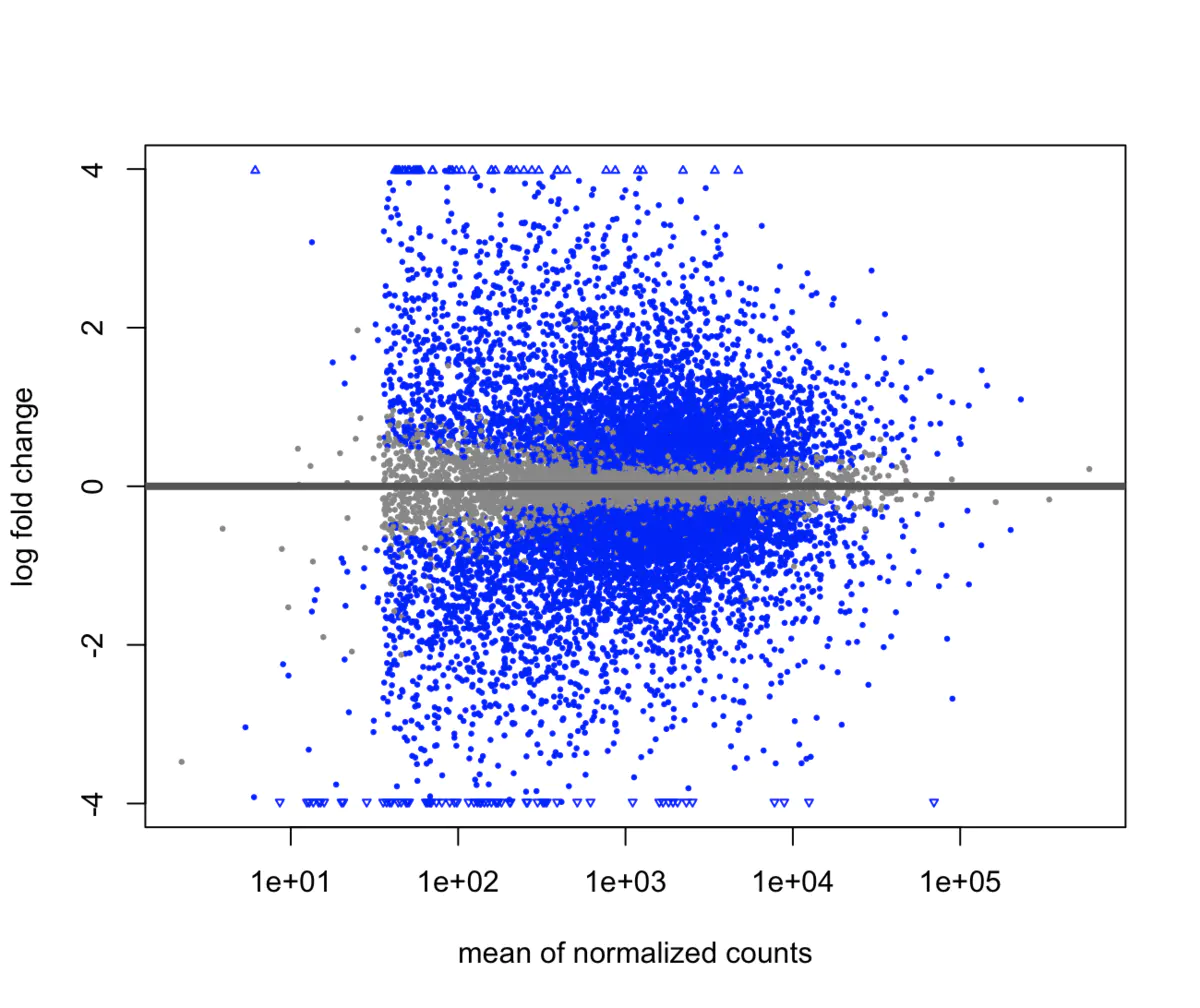 ## 5. 差异基因交集 我们使用 UpSetR 包来对这三种方法所识别出的差异基因进行比较 ```R library(UpSetR) library(RColorBrewer) g.edgeR <- rownames(DEGs.edgeR) g.limma <- rownames(DEGs.limma) g.DESeq2 <- rownames(DEGs.DESeq2) set_list <- list( edgeR = g.edgeR, limma = g.limma, DESeq2 = g.DESeq2 ) upset( fromList(set_list), order.by = "freq", sets.bar.color = brewer.pal(7, "Set2")[1:3], matrix.color = brewer.pal(4, "Set1")[2], main.bar.color = brewer.pal(7, "Set2"), ) ```  或者使用 VennDiagram 绘制韦恩图 ```R library(VennDiagram) grid.newpage() venn_ploy <- venn.diagram( x = list( edgeR = g.edgeR, limma = g.limma, DESeq2 = g.DESeq2 ), filename = NULL, fill = brewer.pal(3, "Set2") ) grid.draw(venn_ploy) ``` 
laihui126
2023年1月12日 17:49
分享文档
收藏文档
上一篇
下一篇
微信扫一扫
复制链接
手机扫一扫进行分享
复制链接
关于 MrDoc
觅道文档MrDoc
是
州的先生
开发并开源的在线文档系统,其适合作为个人和小型团队的云笔记、文档和知识库管理工具。
如果觅道文档给你或你的团队带来了帮助,欢迎对作者进行一些打赏捐助,这将有力支持作者持续投入精力更新和维护觅道文档,感谢你的捐助!
>>>捐助鸣谢列表
微信
支付宝
QQ
PayPal
下载Markdown文件
分享
链接
类型
密码
更新密码